Augmented Dickey-Fuller test

In statistics, an augmented Dickey–Fuller test (ADF) tests the null hypothesis of a unit root in a time series sample. The alternative hypothesis is different depending on which version of the test is used, but is usually stationarity or trend-stationarity. This post explains how to use the ADF test in R, with an attempt to make the different test statistics clear and easily interpretable.

Stationary time series

Roughly, for a time series to be stationary three conditions are needed:

• it shows mean reversion, namely it fluctuates around a constant long-term mean

• it has finite variance that is time-invariant.

• autocorrelations decay relatively fast as lag lenghts increase.

The identification of stationary series can be done by checking whether the autocorrelation function (ACF) drops to zero relatively quickly; usually, the ACF of non-stationary data decreases slowly, and the first-lag value is often large and positive. However, this method is necessarily imprecise, leading to ambiguous situations that cannot be easily deciphered, especially when the sample size is small.

Backshift notation

The backward shift operator \(B\) is defined as follows:

\[ BY_t=Y_{t-1} \]

The operator \(B\) operates on the \(t\)th sample of a time series, with the effect of shifting the sample back one period (first difference). Recall that two applications of the backward shift operator to \(Y_t\) shift the sample back two periods (second difference):

\[ B(BY_t)=B^2Y_t=Y_{t-2} \]

For example, in the case of monthly data, if we wish to consider the same month last year, the notation is \(B^{12}Y_t=Y_{t-12}\).

The backward shift operator is useful to describe the operation of differencing, the technique of election to stabilize the mean value of nonstationary time series by removing changes in the level of a time series, and therefore eliminating (or reducing) trend and seasonality.

A first-order difference is defined as follows:

\[ Y^{\prime}_t=Y_t-Y_{t-1}=Y_t-BY_t=(1-B)Y_t \]

If a second-order difference is considered, namely the first-order difference of a first-order difference, we can write:

\[ \begin{split} Y^{\prime\prime}_t&=Y^{\prime}_t-Y^{\prime}_{t-1}\\ &=(1-B)^2Y_t=Y_t-2BY_t+B^2Y_t\\ &=Y_t-2Y_{t-1}+Y_{t-2} \end{split} \]

A \(d\)-order difference can be written \((1-B)^d\). It is important to note that a second-order difference, denoted by \((1-B)^2\), is not the same as a second difference, which is denoted by \(B^2\).

For example, a seasonal difference followed by a first difference can be written:

\[ \begin{split} Y^{\prime}_t&=(1-B)(1-B^{12})Y_t\\ &=(1-B-B^{12}-B^{13})Y_t\\ &=Y_t-Y_{t-1}-Y_{t-12}-Y_{t-13} \end{split} \]

Sometimes, as I will always do in the following of this post, the notation \(\Delta\) is also used to indicate the first-order difference, i.e., \(\Delta Y_t=(1-B)Y_t\).

A unit root process, also called difference-stationary process (DSP), is a data-generating process whose first difference is stationary.

There are two basic models for time series with linear growth characteristics:

• Trend stationary process

\[ Y_t=c+\delta t+\text{stationary process} \]

• Unit root process

\[ Y_t=Y_{t-1}+\text{stationary process} \]

The processes are indistinguishable for short data records, in the sense that both a trend stationary process (TSP) and a DSP can fit short data records extremely well. However, the processes can be distinguished when restricted to a particular subclass of data-generating processes, such as AR(\(p\)) processes.

Consider the case of an AR(1) process:

\[ Y_t=a_1Y_{t-1}+\epsilon_t \]

We may be interested in testing the hypothesis \(a_1=1\). Since under the null hypothesis the sequence \(\{Y_t\}\) is generated by a nonstationary process, and the variance becomes infinitely large as \(t\) increases, classical statistical methods cannot be used.

Dickey and Fuller devised a procedure to formally test for the presence of a unit root against a number of possible alternatives for explaining the data. It is important to recall that TSP and DSP can produce different forecasts and can give rise to spurious regressions, therefore their detection in time series is a truly important task.

Augmented Dickey-Fuller test

A distinction between stationary and nonstationary time series is made by formal statistical procedures such as the ADF (Augmented Dickey-Fuller) test, which is frequently used since it also accounts for serial correlation in the time series.

Three specifications of the ADF test are based on the following regression equations.

Type 1 (unit root with “none”)

\[ \Delta Y_t=\gamma Y_{t-1}+\underbrace{\sum_{i=2}^p\beta_i\Delta Y_{t-i+1}}_{\text{serial correlation}}+\epsilon_t \tag{1}\]

where \(\epsilon_t\) is white Gaussian noise, stationary with zero mean and constant variance. The statistical hypothesis test is:

\[ (\tau_1)\rightarrow\left\{ \begin{split}H_0:&\quad\gamma=0\\ H_1:&\quad\gamma\neq 0 \end{split} \right. \tag{2}\]

The null hypothesis prescribes the existence of a unit-root in the model. Rejection of the null implies that the original time series does not have a unit root.

Type 2 (unit root with “drift”)

\[ \Delta Y_t=\gamma Y_{t-1}+\underbrace{a_0}_{\text{drift}}+\underbrace{\sum_{i=2}^p\beta_i\Delta Y_{t-i+1}}_{\text{serial correlation}}+\epsilon_t \tag{3}\]

The statistical hypothesis tests are:

\[ \begin{split} &(\phi_1)\rightarrow\left\{ \begin{split}H_0:&\quad\gamma=0\;\text{and}\;a_0=0\\ H_1:&\quad\gamma\neq 0\;\text{ or}\;\;\,a_0\neq0 \end{split} \right.\\ &\\ &(\tau_2)\rightarrow\left\{ \begin{split}H_0:&\quad\gamma=0\\ H_1:&\quad\gamma\neq 0 \end{split} \right. \end{split} \tag{4}\]

Type 3 (unit root with “drift and trend”)

\[ \Delta Y_t=\gamma Y_{t-1}+\underbrace{a_0}_{\text{drift}}+\underbrace{a_2t}_{\text{trend}}+\underbrace{\sum_{i=2}^p\beta_i\Delta Y_{t-i+1}}_{\text{serial correlation}}+\epsilon_t \tag{5}\]

The statistical hypothesis tests are:

\[ \begin{split} &(\phi_2)\rightarrow\left\{ \begin{split}H_0:&\quad\gamma=0\;\text{and}\;a_0=0\;\text{and}\;a_2=0\\ H_1:&\quad\gamma\neq 0\;\text{ or}\;\;\,a_0\neq0\;\text{ or}\;\;\,a_2\neq0\\ \end{split} \right.\\ &\\ &(\phi_3)\rightarrow\left\{ \begin{split}H_0:&\quad\gamma=0\;\text{and}\;a_2=0\\ H_1:&\quad\gamma\neq 0\;\text{ or}\;\;\,a_2\neq0 \end{split} \right.\\ &\\ &(\tau_3)\rightarrow\left\{ \begin{split}H_0:&\quad\gamma=0\\ H_1:&\quad\gamma\neq 0 \end{split} \right. \end{split} \tag{6}\]

Each of the six tests \((\tau_1),(\tau_2),(\tau_3),(\phi_1),(\phi_2),(\phi_3)\) in Equation 2, Equation 4 and Equation 6 corresponds to a progressively more complex linear regression. In all of them there is the root, but in the “drift” model there is also a drift term, and in the “drift and trend” model there are also drift and trend terms. All the coefficients in the models have an associated significance level. While the significance of the root coefficient is the most important and the main focus of the ADF test, we might also be interested in knowing whether or not the drift and trend coefficients are statistically significant.

Summary of the Dickey-Fuller tests

\[ \begin{split} &\begin{split} &\textbf{Trend}\quad\quad\Delta Y_t=\gamma Y_{t-1}+a_0+a_2t+\sum_{i=2}^p\beta_i\Delta Y_{t-i+1}+\epsilon_t\\ &\begin{split} &\text{if}\;(\phi_2)\;\text{is rejected, unit root is NOT present OR there is trend OR there is drift}\\ &\text{if}\;(\phi_2)\;\text{fails to be rejected, unit root is present AND there is NO trend AND there is NO drift}\\ &\text{if}\;(\phi_3)\;\text{is rejected, unit root is NOT present OR there is trend}\\ &\text{if}\;(\phi_3)\;\text{fails to be rejected, unit root is present AND there is NO trend}\\ &\text{if}\;(\tau_3)\;\text{is rejected, unit root is NOT present}\\ &\text{if}\;(\tau_3)\;\text{fails to be rejected, unit root is present}\\ &\end{split} &\end{split}\\ &\begin{split} &\textbf{Drift}\quad\quad\Delta Y_t=\gamma Y_{t-1}+a_0+\sum_{i=2}^p\beta_i\Delta Y_{t-i+1}+\epsilon_t\\ &\begin{split} &\text{if}\;(\phi_1)\;\text{is rejected, unit root is NOT present OR there is drift}\\ &\text{if}\;(\phi_1)\;\text{fails to be rejected, unit root is present AND there is NO drift}\\ &\text{if}\;(\tau_2)\;\text{is rejected, unit root is NOT present}\\ &\text{if}\;(\tau_2)\;\text{fails to be rejected, unit root is present}\\ &\end{split} &\end{split}\\ &\begin{split} &\textbf{None}\quad\quad\Delta Y_t=\gamma Y_{t-1}+\sum_{i=2}^p\beta_i\Delta Y_{t-i+1}+\epsilon_t\\ &\begin{split} &\text{if}\;(\tau_1)\;\text{is rejected, unit root is NOT present}\\ &\text{if}\;(\tau_1)\;\text{fails to be rejected, unit root is present} &\end{split} &\end{split} \end{split} \]

An important extension of the ADF test concerns the case when the noise error term is not white. If the error term is not white and we run the ADF test as it is without accounting for serial correlation, many more rejection of the null tend to be produced than stated at the specified significance level. As the ADF test also deal with the serial correlation by introducing lagged terms, hence we need to select this lag order. This is accomplished by investigating several information criteria, including the autocorrelation function (ACF), but henceforth I limit to use the automatic lag selection functionality provided by the same function of R I will use for running the ADF test. Recall that, in general, the test statistics of the ADF test are very sensitive to changes in the lag structure.

Example

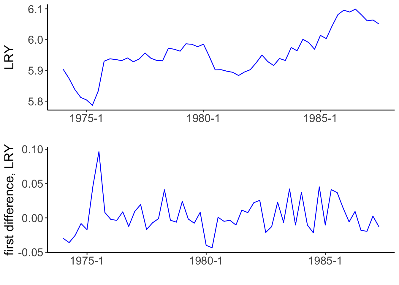
I use functions and data from the urca package. The data set contains the series that S. Johansen and K. Juselius considered for estimating the money demand function of Denmark (Johansen and Juselius 1990). A data frame with quarterly data from Denmark starting in 1974:Q1 until 1987:Q3 contains six variables, including the log real income LRY, whose evolution, together with that of its first difference, is shown in Figure 1.

library(tidyverse)
library(ggpubr)
library(grid)
library(urca)
library(zoo)

data(denmark)
attach(denmark)
denmark <- as.data.frame(denmark)
a <- as.character(ENTRY)
k <- length(a)
for (i in 1:k) substring(a[i], first = 5, last = 5) = "-"
ENTRY <- as.yearqtr(as.factor(a))

df_ts  <- data.frame(x = ENTRY, y = LRY)
df_dts <- data.frame(x = ENTRY[1:k-1], y = diff(LRY))

my_theme = theme(
  axis.title.x = element_text(size = 16),
  axis.text.x = element_text(size = 14),
  axis.title.y = element_text(size = 16),
  axis.text.y = element_text(size = 14),
  legend.title = element_text(size = 14),
  legend.text = element_text(size = 14),
  panel.border = element_blank(),
  panel.grid.major = element_blank(),
  panel.grid.minor = element_blank(),
  panel.background = element_blank(),
  axis.line = element_line(colour = "black"))

p_ts <- ggplot(df_ts, aes(x, y)) +
  geom_line(color = "blue") +
  labs(x = "",
       y = "LRY") + 
  my_theme

p_dts <- ggplot(df_dts, aes(x, y)) +
  geom_line(color = "blue") +
  labs(x = "",
       y = "first difference, LRY") + 
  my_theme

grid.newpage()
grid.draw(rbind(ggplotGrob(p_ts), ggplotGrob(p_dts), size = "last"))

Figure 1: Time series to be tested for stationarity. On the left, the natural logarithm of real income vs. time; on the right its first difference.

The function ur.df() from the urca package performs the ADF test, with three types of models and related tests, named “none” (i.e., Equation 12), “drift” (i.e., Equation 34) and “trend” (Equation 56). The argument selectlags in ur.df() allows to perform automatic selection of the lag structure according to a predefined criterion, as shown in the following code block.

mdl_none_ts   <- ur.df(y = df_ts$y, type = "none", selectlags = c("BIC"))
mdl_drift_ts  <- ur.df(y = df_ts$y, type = "drift", selectlags = c("BIC"))
mdl_trend_ts  <- ur.df(y = df_ts$y, type = "trend", selectlags = c("BIC"))
mdl_none_dts  <- ur.df(y = df_dts$y, type = "none", selectlags = c("BIC"))
mdl_drift_dts <- ur.df(y = df_dts$y, type = "drift", selectlags = c("BIC"))
mdl_trend_dts <- ur.df(y = df_dts$y, type = "trend", selectlags = c("BIC"))
summary(mdl_trend_ts)

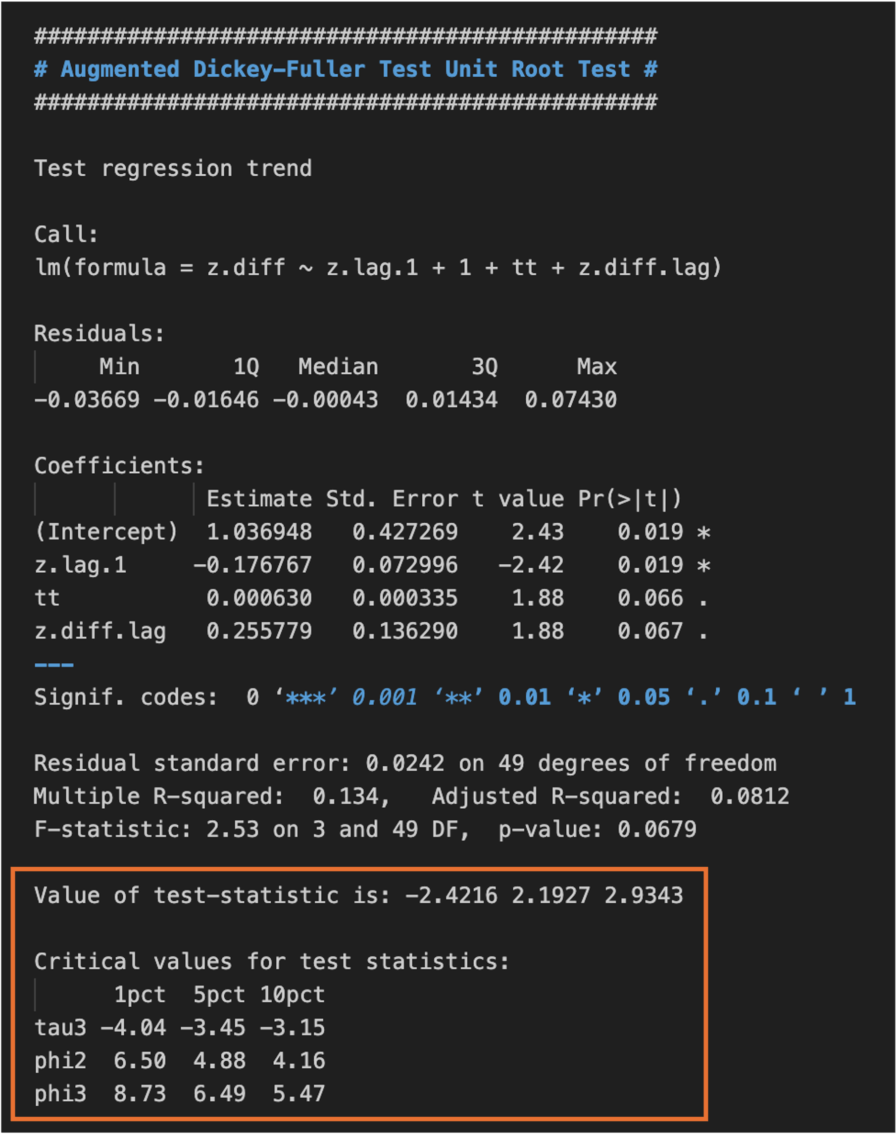
The summary produced when the ADF test is applied to the original time series with the type “trend” is shown in Figure 2.

Figure 2: Results of fitting the “trend” regression model in the ADF test when applied to the `LRY`variable from the `denmark` dataset.

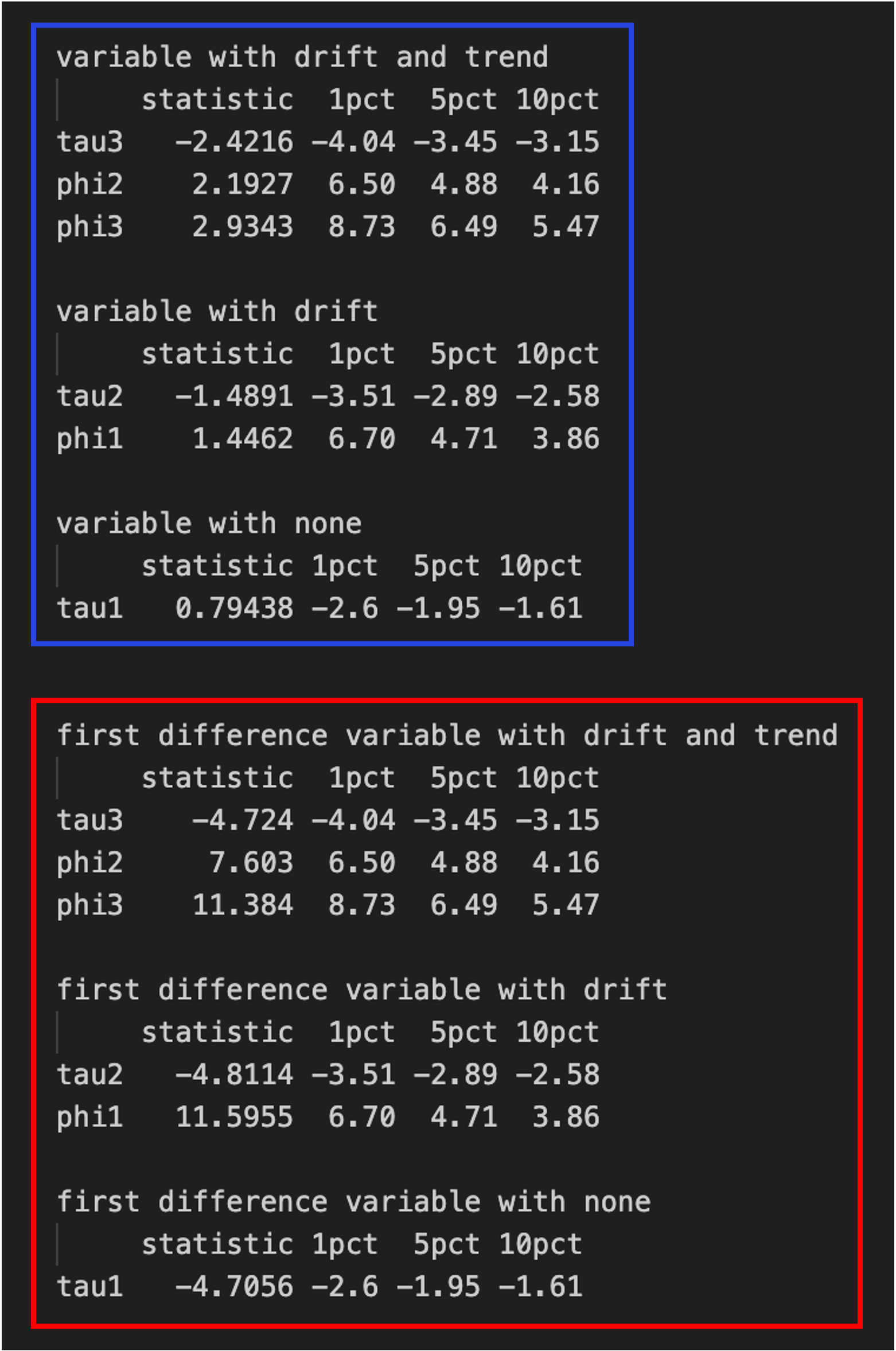
The part of interest for the analysis is within the rectangle highlighted in orange. The “Value of test-statistic is -2.4216 2.1927 2.9343” for tests \((\tau_3), (\phi_2)\) and \((\phi_3)\) are given and the corresponding “Critical values for test statistics” at significance levels 1%, 5% and 10% are reported below, denoted by tau3, phi2 and phi3, respectively. For instance, for the test \((\tau_3)\), given that the test statistic -2.4216 is within the three regions -4.04, -3.45, -3.15 (1%, 5%, 10%) where we fail to reject the null, we do not have evidence to reject the presence of a unit root in the regression model: we can say that there is a unit root. From the \((\phi_2)\)-statistic, the joint null hypothesis is not rejected, therefore there is a unit root AND drift and trend terms are not needed. Similarly, the \((\phi_3)\)-statistic shows that there is a unit root AND a trend term is not needed and the \((\tau_3)\)-statistic shows that there is a unit root. A summary of test results for the variable LRY is reported within the rectangle highlighted in blue in Figure 3.

Figure 3: Results of the three type of ADF tests for the variable `LRY`from the `denmark`dataset.

A close examination of Figure 3 shows that all the tests applied to data of the variable LRY are consistent with failing to reject the corresponding nulls. From the \((\phi_1)\)-statistic, the joint null hypothesis is not rejected, therefore there is a unit root AND the drift term is not needed, and the \((\tau_2)\)-statistic shows that there is a unit root. Finally, the \((\tau_1)\)-statistic also shows that there is a unit root.

On the other hand, all the tests applied to the first difference of the variable LRY reject the corresponding nulls, as shown in the same Figure 3 (summary within the rectangle highlighted in red): although drift and trend terms might be presumed, this variable does not therefore contain a unit root.

Finally, we can conclude that the logarithm of real income contains a unit root and can be a stationary time series by taking the first difference.

References

Johansen, Søren, and Katarina Juselius. 1990. “Maximum Likelihood Estimation and Inference on Cointegration with Applications to the Demand for Money.” Oxford Bulletin of Economics and Statistics 52 (2): 169–210. https://doi.org/10.1111/j.1468-0084.1990.mp52002003.x.